HyperLogLog - Big Data™ in your Browser
In this post we’ll take a look at HyperLogLog, a probabilistic data structure that allows you to estimate the cardinality of huge data sets with minuscule memory requirements. This page is running an implementation JavaScript and uses 4kb to estimate a cardinality of up to 10,000,000 unique visitors based on 50,000,000 randomly generated visits.
What is cardinality? It is the amount of unique elements in a set. And is highly useful for a many problems, e.g. finding the top shared urls or most popular geo locations etc., all based on the amount of how many unique events occurred there.
Probabilistic Data Structures
A nice list of popular probabilistic data structures with case studies can be found in Probabilistic Data Structures for Web Analytics and Data Mining. They can answer a diverse set of problems:
- find most popular elements, e.g. a top 100 list
- estimate the frequency of these elements
- how many elements are in a specified range of data?
- does the data set contain a specific element?
- and, the topic of this post and basis for many of such questions: estimate the cardinality of elements in a set
They work by making smart observations about the internal structure of the data and its correlation with statistical insights. For example HyperLogLog is based on the likelihood of encountering a specific pattern of 0s in the datum and relating that to the size of the cardinality probably necessary to find it. More on that later.
All of them work slightly differently, but what they share is that they trade precision for speed and a (significantly) smaller memory footprint. They are not able to give you the precise answers to the questions above, however, they give acceptable answers at a fraction of the cost.
What is this fraction I talk about? Well in the case of this blog post it’s a 20,000 times smaller memory footprint!
When and Where?
Jump to the TL;DR if you’re already familiar with big data systems.
They usually only make sense when you have high requirements on speed and/or volume. The volume problem can be easily solved via technologies like MapReduce. However when speed is important, specifically with (near) real time requirements one needs to make trade-offs, i.e. either throw more money at the problem or get smarter. This is where probabilistic data structures enter the picture, they are a specific mechanism with specific draw backs and advantages for specific use cases!
First let’s take a quick look at the outline of big data systems. A very nice read on the topic of designing such systems is Big Data: Principles and best practices of scalable realtime data systems by Marz N. and Warren J. Here such a system is categorized broadly as:
\[\text{query} = f(\text{all data})\]Everything else is optimization. And this is good starting point. This idea is highly robust, handles human error well and can use simple to implement and precise algorithms. However, it’s also very slow and expensive! For example, calculating the cardinality like this is pretty straight forward, you just go ahead and count them, without counting the same element twice.
However, in order to deal with real time requirements and make the system usable this view is to simplistic and needs to be augmented. The solution proposed in the book and others is the so called Lambda architecture. This architecture augments the slow but precise Batch layer with an imprecise but efficient Speed layer and a Serving layer that integrates both results to generate a seamless view of the query.
You can find a quick primer and resources on (the aptly named) lambda-architecture.net website that dedicates itself to this architecture.
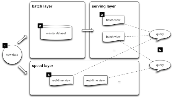 Image owned by lambda-architecture.net
- All data entering the system is dispatched to both the batch layer and the speed layer for processing.
- The batch layer has two functions: (i) managing the master dataset (an immutable, append-only set of raw data), and (ii) to pre-compute the batch views.
- The serving layer indexes the batch views so that they can be queried in low-latency, ad-hoc way.
- The speed layer compensates for the high latency of updates to the serving layer and deals with recent data only.
- Any incoming query can be answered by merging results from batch views and real-time views.
This architecture is not without critique. But it is a good model to keep in your head even if you deviate from this approach.
TL;DR
So, when and where to use probabilistic data structures? If you need to optimize for speed and memory based on (paying) user requirements then add them as mechanism in the speed layer of your architecture. You could argue that doing some preliminary filtering in the serving layer might be a good use case as well, however in my opinion this layer should stay as agnostic to the actual data processing as possible.
HyperLogLog
Theory and implementation notes can be found in HyperLogLog in Practice: Algorithmic Engineering of a State of The Art Cardinality Estimation Algorithm from Research at Google and HyperLogLog: the analysis of a near-optimal cardinality estimation algorithm from Flajolet P., et al., the original authors.
The implementation used in this post is based on this great answer on stackoverflow (what would life be without it) by “actual” which gave me some Aha! moments.
Although the mathematical reasoning behind it is a little bit intricate, the core idea of HyperLogLog is actually quite intuitive. It is based on the likelihood of encountering a specific pattern of 0s in the hash of a datum and relating that to the size of the cardinality probably necessary to find it.
The easiest way to understand it is a slightly different view of the data (without loss of generality). Let’s say the values are viewed as random natural numbers instead of randomized bit vectors, e.g.:
\[\begin{align} 1 &= 0b0000000000000001 \\ 11593 &= 0b0010110101001001 \\ 32768 &= 0b1000000000000000 \\ 44266 &= 0b1010110011101010 \\ 65535 &= 0b1111111111111111 \end{align}\]Half of the randomly chosen numbers will be \(\geq 2^{15}\) (\(2^{16} / 2 = 2^{16} * 2^{-1} = 2^{15}\)). So, the chance to hit a low rank number is very high, e.g. for \(\text{rank}(n) = 1\) (i.e. no leading zero) the chance to hit a number is \(2^{15} / 2^{16} = 50\%\) (a 1 in the front leaving 15 bits). However to find one of \(\text{rank(n)} = 15\) only 1 number is possible, i.e. \(1 = 0b0000000000000001\), so the chance to hit that number is \(1 / 2^{16} = 0.0015\%\).
This is the key observation, the higher the ranks are that you observe the higher the cardinality has to be in order to have enough chances to find it!
Using only this one estimation is very crude however You split your observation into multiple estimators and base the calculation on a mean value of them, more on that in the Implementation.
Now, as I said that example was just a special case. The hashes really are randomly set bit vectors and you can use whatever pattern you want for your rank implementation. However, the shown one is easy to implement and used by the authors.
If you’d rely only on a single measurement you’d introduce a very high variability. Remember, in our example above you had a chance of \(50\%\) to hit a \(rank(n) = 1\), this doesn’t tell you much, cardinality could be anything in \(0 < \text{cardinality} < 2^{15}\). To solve this, a technique known as stochastic averaging used. To that end, the input stream of data elements \(S\) is divided into \(m\) sub streams \(S_i\) of roughly equal size, using the first \(p\) bits of the hash values, where \(m = 2^p\).
This leads us to the actual formula to estimate the cardinality:
\[\begin{align} E &= \alpha_m * m^2 * \left(\sum_{j=1}^{m} 2^{-M[j]}\right)^{-1} \\ M[i] &= \max_{x \in S_i} \text{rank}(x) \end{align}\]The factor \(\alpha_m\) is approximated in real world implementations. For the mathematical details I’d like to refer you to the papers.
Implementation notes
The full code (ECMAScript and transpiled version using Babel) can be found on Github.
You’ll see that a different version for the \(\text{rank}(x)\) function is used. Instead of using the most significant bits, the order is flipped and the least significant bits are used. The implementation of this version is easier and doesn’t make a difference since the hash value is random. Speaking of hash, the FNV-1a hash is used. It is fast and has good randomness.
How did we arrive at the “20,000 times less memory” figure earlier?
The implementation used for the gold standard (actual cardinality) is based on
a hash table: gold[id] = true; with the actual cardinality then being simply
Object.keys(gold).length. Although not the most efficient implementation
memory wise it’s actually well behaved and grows linearly with cardinality. So
assuming a 32 bit architecture:
Why \(4\text{b}\) twice? Well once for the key and once for the value that (a boolean, is represented with an int on x86 when unpacked). So for our cardinality the gold standard needs \(10,000,000 * 8\text{b} \approx 80\text{mb}\). (Note: this is the theoretical minimal size, without taking memory for the object into account.) The HyperLogLog data structure for a standard error of 4% however is using only:
\[\approx 2^{\left\lceil{\log_2\left(\left(\frac{1.04}{0.04}\right)^2\right)}\right \rceil} * 4\text{b} = 4\text{kb}\]Hence \(80\text{mb} = 20,000 * 4\text{kb}\). The size of the HyperLogLog is basically constant, however it doubles as soon as you need to use a 64bit hash for representing bigger (practically unlimited) cardinalities.
The browser experiment uses a Web Worker as driver that generates random visitors and tries to add them as fast as possible to the HyperLogLog and (if the option is checked) the gold implementation. The gold implementation uses the hash table version described earlier. The driver sends updates about the state after specified amount of steps. An interval function is refreshing the graph every second based on the data generated.
| Experiment Parameter | Value |
|---|---|
| Max. Unique Visitors | 10,000,000 |
| Standard Error | 4% |
| Data point every x visits | 10,000 |
| Total visits | 50,000,000 |
| Hash function | FNV-1a |
Run with gold standard?
Then head over to Github and open an Issue please!